


This article appeared first on The Lazy Trader at http://www.the-lazy-trader.com/2012/11/eurusd-donchian-breakout-strategy.html
This article is about a Forex strategy that I designed for the EURUSD currency pair. In this exercise I would like to share with fellow Forex traders the concepts and ideas to take into account in order to design a "likely" long term profitable trading system. Steps to follow in the design process, and methods to find the answers to questions such as "Is there statistical evidence to believe this system has a positive edge?" or "How do I choose a reliable parameter set?" or more important yet "How do I know in the future that the system has possibly stopped working and shouldn't be used anymore?"
The basic idea
The initial idea behind the system is to exploit breakouts. And this is not new at all, many successful methods in the past have successfully exploited these inefficiencies where instead of trying to "Buy low - Sell high" we attempt to "Buy high - Sell higher" or "Sell low - Buy to close even lower".
For example, analyzing the daily time frame. If the price of a currency makes a close today that is higher than every close in the previous X days, then we can say that the currency pair is in an uptrend. At that point we could argue that chances are in favor of a continuation and then we could enter a BUY order betting that we will be able to sell higher in the future. The same for a SHORT trade. If the close today is the lowest close of the last X days, we are in a downtrend and we could enter a SELL order hoping to buy back later at lower prices for a profit.
Of course X, which is the number of days we are going to look back for the lowest close and highest close is a number we need to optimize. The greater the value of X, the stronger the trend has been, but presumably the closest the time for such a trend to be over.
For example X = 80 means we would enter a LONG order if the close yesterday is the highest close of the last 80 days, or a SHORT order if the close yesterday was the lowest of the last 80 days.
X = 80 represents a stronger trend, that is more mature, but also probably coming to an end, we don't know.
A smaller value, for example, X = 50 represents a young potential trend that has been formed. it is not so mature, so chances are lower that it is over, but it could also mean a trend that is not solid yet, and could easily be a fake out.
So, both aproaches have a benefit and a drawback. In the first case, chances are higher that it is a solid and strong trend, but it could also be coming to an end soon, so I might get smaller profits. In the second case I risk entering many fakeouts but if I catch one good trend I'm going to be riding it from the begining, or closer to the begining, thus potentially obtaining more profit from it. But the cost of failing many attempts could affect my overall results.
Profitability of the Parameter space
In any case, what is important to understand is that whether X = 50 or X = 80 give positive results in a back test, that doesn't mean that the idea of designing a strategy based on this principle has any merit. For the idea to be truly validated as potentially good, positive results need to be obtained for the neighborhood of surrounding parameters. Let's say X = 80 gives you positive returns on a 10 year backtest, but X = 78, or X = 82 give loses? That means, you probably just curve fitted your system and the system will fail at the slightest market mutation in the future.
That's why we need to verify that surrounding parameters of the space also yield positive results. So, below is a simple Optimization Test from 01/01/2000 to 31/12/2009 run in Metatrader 4, entering trades for 50 day break outs, 55, 60, 65, 70, 75, 80, 85, 90, 95 and 100 day break outs combined with time based exits 6 days to 12 days after the entry.
(Click on image to enlarge)

The darker the rectangles the higher the profit obtained in the ten year back-test. White rectangles mean negative profits, that is loses. As you can see all the combinations of parameters yield profits in 10 year back-tests (All green rectangles and no white ones). This means, if you were to choose a given combination and the market mutates, you won't be drastically affected in the future because you have a strong parameter space to withstand market variations. So even though you might not trade with the optimal parameter set in the future you are still bound to have odds in your favor because you are likely trading a parameter set that although is not the optimal anymore, at least it is a profitable one.
I like the combination of 70 day break out with 6 days time based exit. It is not the one that yields the highest profit in the 10 year optimization report, not at all. But it is the one with the best ratio of AverageAnnualReturn/MaximumDrawDown. That's the AAR/MDD ratio. It combines a decent return with one of the smallest Drawdowns in the parameter space and I like that, small draw downs whenever possible.
Positive Mathematical Expectancy of the Entry
We need to make sure that our entry logic is better than a random entry. For that we analyze every single entry in the ten year period and compile the Average Maximum Favorable Excursion (MFE) and the Average Maximum Adverse Excursion (MAE). For more information about what MFE and MAE are, how they are calculated take a look at my article How to measure a system's edge. It is all explained there.
The Mathematical Expectancy Analysis reveals that for the 70 day break out with 6 days time based exit there were 363 entries (363 trades). The Average Maximum Favorable Excursion (MFE) was 160.84 and The Average Maximum Adverse Excursion (MAE) was 121.77. That means, on average trades went in our favor by a distance of 160.84% of the daily ATR and against us by a distance equal to 121.77% of the ATR while we were on the trades (6 days for each trade).
We can see that MFE is greater than MAE, so our entry has a positive edge. Trades went, on average, farther in our favor than against us. This edge can be measured with the Edge Ratio dividing MFE/MAE = 1.32
A truly random entry has an Edge Ratio of 1.00. Our entry has an edge ratio of 1.32 which is a signifficant edge. Our entry logic has a positive edge.
Analyzing our Exit's Edge
But we also need to verify that this is not a lucky occurrence. So, ideally the Edge Ratio is higher than 1.00 not only for the 6 days exit, but for the surroundings. For example the edge ratio should be > 1.00 for 4 days exits and for 8 days exits as well. Back to the calculation again and we obtain:
We now have a strong evidence to believe that both our entries and exits have a positive edge and that the parameter space is wide enough to show profitability with different parameter sets. We won't be simply choosing a set of specific unique parameters that happened to yield positive returns in the past.
Setting Targets and Stop Losses with Walk Forward Analysis and Rank Parameter selection
Now, we need to define a Target Profit and Stop Loss for our trades. These values won't be a hard number of pips, because hard number of pips won't be useful when the volatility of the currencies changes. Our distance to Target Point and Stop Loss will be variable and based on currently volatility. That's why we will set them as a percentage of the Average True Range (ATR) at the time of the entry.
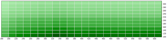
We run another optimization where we combine possible Targets from 180% of the ATR to 600% of the ATR combined with Stop Losses from 100% of the ATR to 300% of the ATR. And we cover the parameters space coarsely, using 20% steps.
(Click on image to enlarge)
We run several optimization reports in two year intervals as follows:
1/1/2000 to 31/12/2001
1/1/2001 to 31/12/2002
1/1/2002 to 31/12/2003
1/1/2003 to 31/12/2004
1/1/2004 to 31/12/2005
1/1/2005 to 31/12/2006
1/1/2006 to 31/12/2007
1/1/2007 to 31/12/2008
1/1/2008 to 31/12/2009
The idea is to obtain the parameter combination of TP and SL that yields the most stable dradown values and the most stable yearly returns. We don't care about the highest return, because there is no guarantee that such parameter set will give the highest return in the future. We want to prioritize stability (Smallest standard deviation of the yearly returns, and drawdowns). We simply want the parameter set with the smallest variability.
We have a bunch of good candidates but the two most stable parameters sets are:
Target 320 % of the ATR, Stop Loss 200 % of the ATR
Target 340 % of the ATR, Stop Loss 200 % of the ATR
The first one is a bit more stable, it has a slightly higher return and a slightly lower maximum draw-down so I'm sticking with that one.
Finally we run a back test of our most stable parameter set for the optimization period 2000 - 2009 and this is what we get:
(Click on image to enlarge)

Yearly returns
2000 +8.55%
2001 +3.40%
2002 +17.28%
2003 +19.69%
2004 +10.60%
2005 -0.96%
2006 +12.27%
2007 +8.09%
2008 +12.42%
2009 -2.28%
We have obtained a strategy with a positive mathematical expectancy, a wide profitable parameter space and we determined the most stable combination for setting Targets and Stop Losses.
The strategy enters orders with a 70 day break out of the highest close or the lowest close. We set a Target equal to 320% of the ATR which we calculate in terms of pips at the time of our entry based on the value of the ATR at the moment, and we also set a Stop Loss at a distance of 200% of the ATR. This way our strategy is flexible to volatilty changes in the currency pair. Finally if our TP or SL is not hit, we exit the trade 6 days after the entry.
Some additional statistics:
Average Annual Return : 8.90%
Maximum Drawdown : 9.75%
AAR/MDD : 0.91
Ulcer Index : 3.23
Sharpe Ratio : 1.13
Martin Ratio : 2.38
When to stop trading the system?
This is perhaps the most important question because it will give you confidence to stick to the system in the inevitable bad times, and only stop using it when there is evidence that the strategy stopped working. And obviously realize it before your account has suffered a significant draw down.
The fact that the system had a maximum draw down of 9.75% doesn't mean that a higher value won't happen in the future. But we need to decide how much more pain we are willing to suffer before we decide that the system stopped working.
In order to accomplish this we use Monte Carlo simulations. Essentially we distribute all the outcomes of our past trades in different orders. All the losses and winners distributed randomly and not in the particular order in which they took place in the past. We distribute all 363 trades randomly and we do it 100 000 times. That introduces enough randomness in the possible orders or combinations in which the sequence of losses and wins may happen. Then for all 100 000 combinations we analyze final profits and draw downs. We then assume that if our trading in real life reaches the worst Monte Carlo scenarios in terms of profits and draw downs the system has stopped working and it is not safe to use anymore because presumably, the market inefficiency that it exploited is not present anymore.
After analyzing the 100 000 iteration Monte Carlo simulation we obtain the following values:
Worse Case Draw-down 17.63%
Worst case consecutive losses 19
If our system reaches a 17.63% draw-down we can stop using it with evidence suggesting that most likely it has stopped working. As well as if it reaches 19 consecutive losses.
At this point we are done designing our likely long term profitable system. Which we designed and optimized using 2000 - 2009 data. Aren't you curious to know how the system performed during 2010 - 2012?
2010 - 2012 will be our out of sample testing period. Essentially simulating how the system would have traded life from 2010 to 2012 which is a period totally alien and unknown for a system designed using only data from 2000 to 2009.
According to the characteristics of the system, we can expect an average yearly return of 8.90% with a standard deviation of 6.83.
That means there is:
- A 68% chance that our yearly return will be between 2.07% and 15.73%.
- A 95% chance that our yearly return will be between -4.76% and 22.76%
Without further ado here are the results:
2010 +6.12%
2011 -4.27%
2012 +7.83%
Our yearly returns are within the expected intervals. We have one negative year in 2010 but there is no evidence that the system stopped working given that our worst case draw down scenario hasn't happened. The system performs better in 2012 and we obtain a 7.83% return for 2012. Overall a 9.54% equity growth is obtained between 2010 and 2012 with a maximum draw down of 8.51%.
Of course if you want to increase your returns you increase your risk per trade. All the simulations were done with 1% risk per trade, calculating the position size accordingly so that if SL was hit, only 1% of the account was lost. If you increase the risk level to 2% per trade you can expect to double everything, both profits and draw downs. You would have achieved 17.80% average yearly returns in the 2000-2009 period but also a 19.50% maximum draw-down and the worst Monte Carlo scenario would be a 35.26% draw down. What matters in the end is the AAR/MDD ratio (which is always 0.91). It is up to the trader to decide how aggressive he wants to be with his risks per trade levels.
The strategy doesn't use unsound trading principles such as Martingale or Grid trading. It has a positive mathematical expectancy and a wide parameter space of consistently long term profitable parameters. It is not the flashiest or most spectacular strategy in the world, but it is a profitable one nonetheless and a strategy that has been working for the past 12 years, with evidence suggesting that it hasn't stopped working. For sure, I will revisit it at the end of 2013 to analyze its trading results from January 2013 to December 2013.
I hope this article shines some light on the design principles of mechanical Forex systems, or any mechanical system for that matter and that it helps some one out there.
Download source code of the Expert - Lazy Trader Breakout EA
This article appeared first on The Lazy Trader at http://www.the-lazy-trader.com/2012/11/eurusd-donchian-breakout-strategy.html
- The simulations have been run in Metatrader 4, with AlpariUK data directly provided by the broker.
- A 2 pip fixed spread was set using the Spread Fixer tool implemented by Asirikuy.com
- The Mathematical Expectancy Analysis was carried out using Asirikuy's Mathematical Expectancy Analysis tool
- The Walk Forward Analysis along with the Parameters Rank Analysis, the Analysis of yearly returns and draw-downs as well as the system's characteristics were obtained using Asirikuy's Draw down Analysis Tool.
- The Monte Carlo simulations were run using Asirikuy's Monte Carlo simulator.
Results - 2014
Results - 2015
Results - 2016
Related Articles:
How to measure a system's edge
Position Size Calculator for Metatrader
Tips for reviewing Expert Advisors
Trading with realistic expectations
Forex Cash Cow. Review and Expert Advisor
LT Trend Sniper - A Forex strategy that works
The Turtles Trading system automated (Expert Advisor for download)
Useful resources for learning about mechanical trading systems
Go to the bottom of this page in order to see the Legal Stuff
This article is about a Forex strategy that I designed for the EURUSD currency pair. In this exercise I would like to share with fellow Forex traders the concepts and ideas to take into account in order to design a "likely" long term profitable trading system. Steps to follow in the design process, and methods to find the answers to questions such as "Is there statistical evidence to believe this system has a positive edge?" or "How do I choose a reliable parameter set?" or more important yet "How do I know in the future that the system has possibly stopped working and shouldn't be used anymore?"
The basic idea
The initial idea behind the system is to exploit breakouts. And this is not new at all, many successful methods in the past have successfully exploited these inefficiencies where instead of trying to "Buy low - Sell high" we attempt to "Buy high - Sell higher" or "Sell low - Buy to close even lower".
For example, analyzing the daily time frame. If the price of a currency makes a close today that is higher than every close in the previous X days, then we can say that the currency pair is in an uptrend. At that point we could argue that chances are in favor of a continuation and then we could enter a BUY order betting that we will be able to sell higher in the future. The same for a SHORT trade. If the close today is the lowest close of the last X days, we are in a downtrend and we could enter a SELL order hoping to buy back later at lower prices for a profit.
Of course X, which is the number of days we are going to look back for the lowest close and highest close is a number we need to optimize. The greater the value of X, the stronger the trend has been, but presumably the closest the time for such a trend to be over.
For example X = 80 means we would enter a LONG order if the close yesterday is the highest close of the last 80 days, or a SHORT order if the close yesterday was the lowest of the last 80 days.
X = 80 represents a stronger trend, that is more mature, but also probably coming to an end, we don't know.
A smaller value, for example, X = 50 represents a young potential trend that has been formed. it is not so mature, so chances are lower that it is over, but it could also mean a trend that is not solid yet, and could easily be a fake out.
So, both aproaches have a benefit and a drawback. In the first case, chances are higher that it is a solid and strong trend, but it could also be coming to an end soon, so I might get smaller profits. In the second case I risk entering many fakeouts but if I catch one good trend I'm going to be riding it from the begining, or closer to the begining, thus potentially obtaining more profit from it. But the cost of failing many attempts could affect my overall results.
Profitability of the Parameter space
In any case, what is important to understand is that whether X = 50 or X = 80 give positive results in a back test, that doesn't mean that the idea of designing a strategy based on this principle has any merit. For the idea to be truly validated as potentially good, positive results need to be obtained for the neighborhood of surrounding parameters. Let's say X = 80 gives you positive returns on a 10 year backtest, but X = 78, or X = 82 give loses? That means, you probably just curve fitted your system and the system will fail at the slightest market mutation in the future.
That's why we need to verify that surrounding parameters of the space also yield positive results. So, below is a simple Optimization Test from 01/01/2000 to 31/12/2009 run in Metatrader 4, entering trades for 50 day break outs, 55, 60, 65, 70, 75, 80, 85, 90, 95 and 100 day break outs combined with time based exits 6 days to 12 days after the entry.
(Click on image to enlarge)

The darker the rectangles the higher the profit obtained in the ten year back-test. White rectangles mean negative profits, that is loses. As you can see all the combinations of parameters yield profits in 10 year back-tests (All green rectangles and no white ones). This means, if you were to choose a given combination and the market mutates, you won't be drastically affected in the future because you have a strong parameter space to withstand market variations. So even though you might not trade with the optimal parameter set in the future you are still bound to have odds in your favor because you are likely trading a parameter set that although is not the optimal anymore, at least it is a profitable one.
I like the combination of 70 day break out with 6 days time based exit. It is not the one that yields the highest profit in the 10 year optimization report, not at all. But it is the one with the best ratio of AverageAnnualReturn/MaximumDrawDown. That's the AAR/MDD ratio. It combines a decent return with one of the smallest Drawdowns in the parameter space and I like that, small draw downs whenever possible.
Positive Mathematical Expectancy of the Entry
We need to make sure that our entry logic is better than a random entry. For that we analyze every single entry in the ten year period and compile the Average Maximum Favorable Excursion (MFE) and the Average Maximum Adverse Excursion (MAE). For more information about what MFE and MAE are, how they are calculated take a look at my article How to measure a system's edge. It is all explained there.
The Mathematical Expectancy Analysis reveals that for the 70 day break out with 6 days time based exit there were 363 entries (363 trades). The Average Maximum Favorable Excursion (MFE) was 160.84 and The Average Maximum Adverse Excursion (MAE) was 121.77. That means, on average trades went in our favor by a distance of 160.84% of the daily ATR and against us by a distance equal to 121.77% of the ATR while we were on the trades (6 days for each trade).
We can see that MFE is greater than MAE, so our entry has a positive edge. Trades went, on average, farther in our favor than against us. This edge can be measured with the Edge Ratio dividing MFE/MAE = 1.32
A truly random entry has an Edge Ratio of 1.00. Our entry has an edge ratio of 1.32 which is a signifficant edge. Our entry logic has a positive edge.
Analyzing our Exit's Edge
But we also need to verify that this is not a lucky occurrence. So, ideally the Edge Ratio is higher than 1.00 not only for the 6 days exit, but for the surroundings. For example the edge ratio should be > 1.00 for 4 days exits and for 8 days exits as well. Back to the calculation again and we obtain:
| MFE | MAE | Edge Ratio | |
| 4 day exit | 125.29 | 100.26 | 1.25 |
| 6 day exit | 160.84 | 121.77 | 1.32 |
| 8 day exit | 189.41 | 138.55 | 1.34 |
We now have a strong evidence to believe that both our entries and exits have a positive edge and that the parameter space is wide enough to show profitability with different parameter sets. We won't be simply choosing a set of specific unique parameters that happened to yield positive returns in the past.
Setting Targets and Stop Losses with Walk Forward Analysis and Rank Parameter selection
Now, we need to define a Target Profit and Stop Loss for our trades. These values won't be a hard number of pips, because hard number of pips won't be useful when the volatility of the currencies changes. Our distance to Target Point and Stop Loss will be variable and based on currently volatility. That's why we will set them as a percentage of the Average True Range (ATR) at the time of the entry.
We run another optimization where we combine possible Targets from 180% of the ATR to 600% of the ATR combined with Stop Losses from 100% of the ATR to 300% of the ATR. And we cover the parameters space coarsely, using 20% steps.
(Click on image to enlarge)

We run several optimization reports in two year intervals as follows:
1/1/2000 to 31/12/2001
1/1/2001 to 31/12/2002
1/1/2002 to 31/12/2003
1/1/2003 to 31/12/2004
1/1/2004 to 31/12/2005
1/1/2005 to 31/12/2006
1/1/2006 to 31/12/2007
1/1/2007 to 31/12/2008
1/1/2008 to 31/12/2009
The idea is to obtain the parameter combination of TP and SL that yields the most stable dradown values and the most stable yearly returns. We don't care about the highest return, because there is no guarantee that such parameter set will give the highest return in the future. We want to prioritize stability (Smallest standard deviation of the yearly returns, and drawdowns). We simply want the parameter set with the smallest variability.
We have a bunch of good candidates but the two most stable parameters sets are:
Target 320 % of the ATR, Stop Loss 200 % of the ATR
Target 340 % of the ATR, Stop Loss 200 % of the ATR
The first one is a bit more stable, it has a slightly higher return and a slightly lower maximum draw-down so I'm sticking with that one.
Finally we run a back test of our most stable parameter set for the optimization period 2000 - 2009 and this is what we get:
(Click on image to enlarge)

Yearly returns
2000 +8.55%
2001 +3.40%
2002 +17.28%
2003 +19.69%
2004 +10.60%
2005 -0.96%
2006 +12.27%
2007 +8.09%
2008 +12.42%
2009 -2.28%
We have obtained a strategy with a positive mathematical expectancy, a wide profitable parameter space and we determined the most stable combination for setting Targets and Stop Losses.
The strategy enters orders with a 70 day break out of the highest close or the lowest close. We set a Target equal to 320% of the ATR which we calculate in terms of pips at the time of our entry based on the value of the ATR at the moment, and we also set a Stop Loss at a distance of 200% of the ATR. This way our strategy is flexible to volatilty changes in the currency pair. Finally if our TP or SL is not hit, we exit the trade 6 days after the entry.
Some additional statistics:
Average Annual Return : 8.90%
Maximum Drawdown : 9.75%
AAR/MDD : 0.91
Ulcer Index : 3.23
Sharpe Ratio : 1.13
Martin Ratio : 2.38
When to stop trading the system?
This is perhaps the most important question because it will give you confidence to stick to the system in the inevitable bad times, and only stop using it when there is evidence that the strategy stopped working. And obviously realize it before your account has suffered a significant draw down.
The fact that the system had a maximum draw down of 9.75% doesn't mean that a higher value won't happen in the future. But we need to decide how much more pain we are willing to suffer before we decide that the system stopped working.
In order to accomplish this we use Monte Carlo simulations. Essentially we distribute all the outcomes of our past trades in different orders. All the losses and winners distributed randomly and not in the particular order in which they took place in the past. We distribute all 363 trades randomly and we do it 100 000 times. That introduces enough randomness in the possible orders or combinations in which the sequence of losses and wins may happen. Then for all 100 000 combinations we analyze final profits and draw downs. We then assume that if our trading in real life reaches the worst Monte Carlo scenarios in terms of profits and draw downs the system has stopped working and it is not safe to use anymore because presumably, the market inefficiency that it exploited is not present anymore.
After analyzing the 100 000 iteration Monte Carlo simulation we obtain the following values:
Worse Case Draw-down 17.63%
Worst case consecutive losses 19
If our system reaches a 17.63% draw-down we can stop using it with evidence suggesting that most likely it has stopped working. As well as if it reaches 19 consecutive losses.
At this point we are done designing our likely long term profitable system. Which we designed and optimized using 2000 - 2009 data. Aren't you curious to know how the system performed during 2010 - 2012?
2010 - 2012 will be our out of sample testing period. Essentially simulating how the system would have traded life from 2010 to 2012 which is a period totally alien and unknown for a system designed using only data from 2000 to 2009.
According to the characteristics of the system, we can expect an average yearly return of 8.90% with a standard deviation of 6.83.
That means there is:
- A 68% chance that our yearly return will be between 2.07% and 15.73%.
- A 95% chance that our yearly return will be between -4.76% and 22.76%
Without further ado here are the results:
2010 +6.12%
2011 -4.27%
2012 +7.83%
Our yearly returns are within the expected intervals. We have one negative year in 2010 but there is no evidence that the system stopped working given that our worst case draw down scenario hasn't happened. The system performs better in 2012 and we obtain a 7.83% return for 2012. Overall a 9.54% equity growth is obtained between 2010 and 2012 with a maximum draw down of 8.51%.
Of course if you want to increase your returns you increase your risk per trade. All the simulations were done with 1% risk per trade, calculating the position size accordingly so that if SL was hit, only 1% of the account was lost. If you increase the risk level to 2% per trade you can expect to double everything, both profits and draw downs. You would have achieved 17.80% average yearly returns in the 2000-2009 period but also a 19.50% maximum draw-down and the worst Monte Carlo scenario would be a 35.26% draw down. What matters in the end is the AAR/MDD ratio (which is always 0.91). It is up to the trader to decide how aggressive he wants to be with his risks per trade levels.
The strategy doesn't use unsound trading principles such as Martingale or Grid trading. It has a positive mathematical expectancy and a wide parameter space of consistently long term profitable parameters. It is not the flashiest or most spectacular strategy in the world, but it is a profitable one nonetheless and a strategy that has been working for the past 12 years, with evidence suggesting that it hasn't stopped working. For sure, I will revisit it at the end of 2013 to analyze its trading results from January 2013 to December 2013.
I hope this article shines some light on the design principles of mechanical Forex systems, or any mechanical system for that matter and that it helps some one out there.
Download source code of the Expert - Lazy Trader Breakout EA
This article appeared first on The Lazy Trader at http://www.the-lazy-trader.com/2012/11/eurusd-donchian-breakout-strategy.html
- The simulations have been run in Metatrader 4, with AlpariUK data directly provided by the broker.
- A 2 pip fixed spread was set using the Spread Fixer tool implemented by Asirikuy.com
- The Mathematical Expectancy Analysis was carried out using Asirikuy's Mathematical Expectancy Analysis tool
- The Walk Forward Analysis along with the Parameters Rank Analysis, the Analysis of yearly returns and draw-downs as well as the system's characteristics were obtained using Asirikuy's Draw down Analysis Tool.
- The Monte Carlo simulations were run using Asirikuy's Monte Carlo simulator.
Results - 2014
Results - 2015
Results - 2016
Related Articles:
How to measure a system's edge
Position Size Calculator for Metatrader
Tips for reviewing Expert Advisors
Trading with realistic expectations
Forex Cash Cow. Review and Expert Advisor
LT Trend Sniper - A Forex strategy that works
The Turtles Trading system automated (Expert Advisor for download)
Useful resources for learning about mechanical trading systems
Go to the bottom of this page in order to see the Legal Stuff
Excellent work! Thanks for sharing this!
ReplyDeleteIt is not the flashiest or most spectacular strategy in the world, but it is a profitable one nonetheless and a strategy that has been working for the past 12 years, with evidence suggesting that it hasn't stopped working.feng shui
ReplyDeleteThanks for sharing! Unfortunately it is not working for me with build 600. Hopefully just me?
ReplyDeleteHi heath,
ReplyDeleteFor build 600 you have to copy the expert in a different folder. Go to File -> Open Data Folder, that will open the new data location of your MT4 station in computer browser. Once there, copy the expert inside the Experts directory that you see in that location. Restart your MT4.
Cheers,
LT
That is probably the most useful thing I have ever read about trading systems ever! Thanks for sharing
ReplyDeleteExcellent analysis, I just stumbled on this site and this particular page was really in depth on how to construct and evaluate a mechanical system. Do we consider this system still workable? In the year 2014 (this year) it seems that the system went through a drawdown of 40% and 28 consecutive losses before recovering it's previous equity high. the monte carlo simulations suggest that 17.63% and 19 consecutive losses should be the worst this system gets right?
ReplyDeleteNop, according to my analysis the system is up +5.33% this year. with 25 wins and 14 losses.
DeleteIt is unlikely to suffer 28 losses in a row in just one year as it trades on the daily time frames. So trades are no frequent. Aren't you perhaps testing on another time-frame? H1 perhaps by mistake? This is a daily system.
Regards,
LT
You're right, I did make this silly mistake. I should have checked, sorry about that!
ReplyDeleteIs there any advantage of trading this over many pairs simultaneously or even commodities etc ??
ReplyDeleteYou will get increased DD and account vol but would it make any more profit ?
Wow, I think this simpler strategy looks even better than one used by your "LT Trend Sniper" EA, at least on paper (only talking about average annual ROI and DD and trading EURUSD as the single currency pair)... look:
ReplyDeleteRisk Per Trade: 1%; Average Annual Return: 8.90%; Maximum Drawdown: -9.75% (LT Trend Sniper).
vs
Risk Per Trade: 1%; Average Annual Return: 3.29%; Maximum Drawdown: -3.01% (50Day-Breakout).
...
According to the Manual, we would need to risk almost 3% per trade in order to have similar returns and DD (9.96 and -8.80 respectively):
Am I correct, Henrik? What's your opinion about it?
Hey Victor,
Deletethe 8.90 annual return vs 9.75 MDD are not sniper numbers. Those are this article's strategy's numbers. The Sniper has a better AAR/MDD ratio. And it is more stable. Meaning, smaller standard deviation of the annual returns, smaller standard deviation of annual draw-downs. Greater number of positive years.
LT
Henrik,
DeleteYou're right! It was just a typo... I meant the opposite:
Risk Per Trade: 1%; Average Annual Return: 8.90%; Maximum Drawdown: -9.75% (50Day-Breakout)... vs... Risk Per Trade: 1%; Average Annual Return: 3.29%; Maximum Drawdown: -3.01% or Risk Per Trade: 3%; Average Annual Return: 9.96%; Maximum Drawdown: -8.80% (LT Trend Sniper).
I would generally assume that trading with smaller position sizing for obtaining the same or similar results, is a better idea, because then you can better "escalate" returns (of course with their corresponding DD).
Could you please elaborate little more on that?
Of course! To me AAR/MDD ratio is all that matters in the end. The higher the better. By the way notice how the typical AAR/MDD ratio for professional audited traders is usually around 0.5 http://www.barclayhedge.com/research/indices/cta/sub/curr.html
DeleteLT
Great comparison! Other than the amount being managed, I strongly believe there's too much bias regarding what truly makes a "professional" ¬¬... And yes, I definitely need to study more about the differences between the future potential of the EAs we are discussing.
DeleteVíctor
This comment has been removed by the author.
ReplyDelete